The Machine Language

In this section, we will look into the language understood by the processor - the machine language - and present how the processor executes a program.

As discussed in the previous section, each processor is able to execute a particular set of instructions, depending on its ISA. But how do we actually talk to the processor, telling it which instructions it should execute? While as (future) engineers, we mostly think of algorithms and programs in a symbolic form (including types and variables), the processor at the hardware level has no idea of such things. It only understands instructions in a very concrete form, called the machine language, in binary format: ones and zeros.

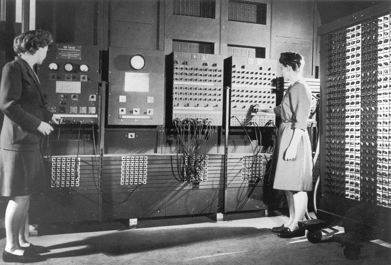
In ancient times, this was more or less the level of abstraction on which computers were programmed: By connecting cables and setting switches. The photo above shows two programmers (Betty Jean Jennings and Fran Bilas) operating the ENIAC computer in 1946.

From a high level language to machine language

Nowadays, nobody would want to write machine language any more. Instead, we write programs in dedicated languages such as C or OCaml. A special program -- the compiler -- is used to translate programs from high level languages down to the machine language of a specific target architecture. We will not go into the details of the compilation process here¹, you will learn more about it later in this and other lectures. But let's have a quick look at the different levels of abstraction.

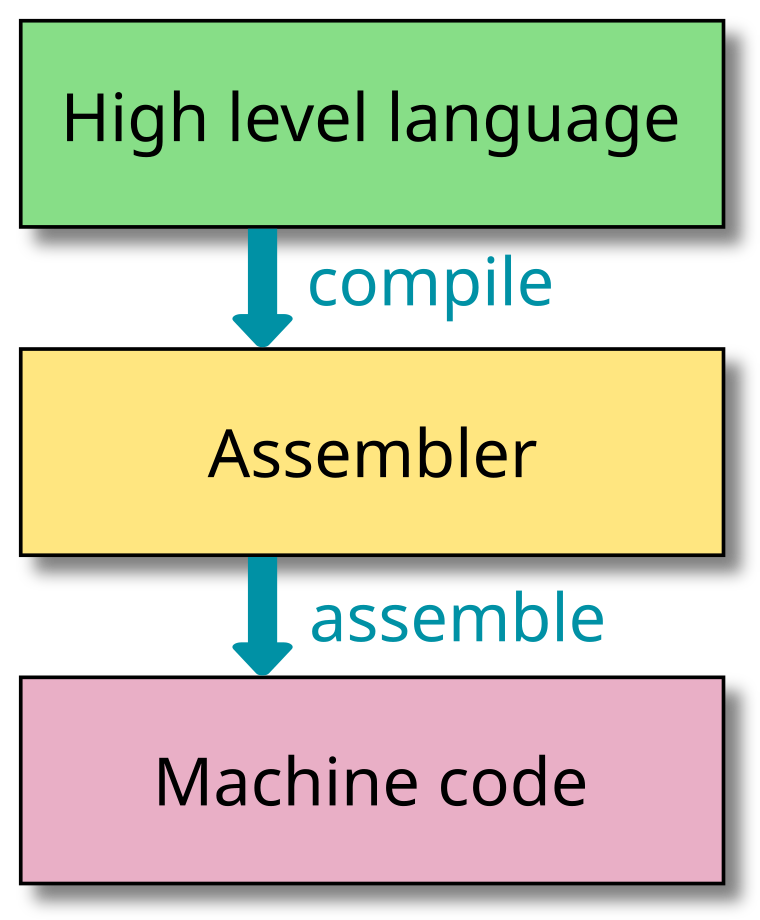
The above figure shows the basic steps in the compilation: We are starting from a high level programming language. At this point, the program is given in an abstract form: It does not know about the concrete hardware architecture it will run on. This has the advantage that programs written in a programming language are mostly portable: They can be run on computers with different ISAs. The basic elements in most programming languages are variables and functions. As an example, here is a small snippet of C:

int square(int x) {
    return x * x;
}

int main() {
    int x = square(42);
}

Without diving into the concrete syntax of C, this program basically computes the square of 42, which you have probably guessed without much of a headache. The first step is compilation, which translates the generic code to another language, called assembler. While the assembler code is still human readable, the representation is already specific to a certain ISA: It uses mnemonic forms of the ISA's instructions and registers, symbolic labels, as well as different textual representations of literals (constant values):

square:
   addi  sp,sp,-16
   sw    ra,12(sp)
   sw    s0,8(sp)
   addi  s0,sp,16
   sw    a0,-16(s0)
   lw    a1,-16(s0)
   lw    a0,-16(s0)
   call  __mulsi3
   mv    a5,a0
   mv    a0,a5
   lw    ra,12(sp)
   lw    s0,8(sp)
   addi  sp,sp,16
   jr    ra
   .align   2
main:
   addi  sp,sp,-16
   sw    ra,12(sp)
   sw    s0,8(sp)
   addi  s0,sp,16
   li    a0,42
   call  square
   sw    a0,-16(s0)
   li    a5,0
   mv    a0,a5
   lw    ra,12(sp)
   lw    s0,8(sp)
   addi  sp,sp,16
   jr    ra

The above code shows the same program in RISC-V assembler. There are two labels (main and square), otherwise there is one instruction per line of code. Each instruction starts with the instruction name (such as addi), followed by its arguments. The arguments can be one or more registers (such as a0 or sp), a constant, or a label, depending on the instruction. There is a fixed number of registers, each of which can hold 32 bits of data: function arguments, intermediate results, return values, or addresses. The registers constitute the working memory of the processor. They have no type, the programmer needs to know which kind of data she is manipulating.

The second step in the compilation process -- also called assembler -- resolves any symbolic labels and directives and produces the final machine code. Here is a hexadecimal representation of the machine code for the above program:

ff010113  00112623  00812423  01010413 
fea42823  ff042583  ff042503  00000097 
000080e7  00050793  00078513  00c12083 
00812403  01010113  00008067  ff010113 
00112623  00812423  01010413  02a00513 
00000097  000080e7  fea42823  00000793 
00078513  00c12083  00812403  01010113 
00008067                               

Instruction types

Looking back at the assembler code that resulted from the compilation of the squaring program, we find different types of instructions, each of which accomplishes a simple task. A first class of instructions are those performing arithmetic and logic operations. Examples are addition (such as the addi instruction in the code), subtraction, bitwise and, or bit shifting to the left.

A second class of instructions are memory access instructions, which move data from and to the memory. Load instructions fetch data from the memory to a register, while store instructions do the reverse: saving the value of a register to a given memory addresss. Examples in the assembler code are the lw (load word) and sw (store word) instructions.

A third class is formed by instructions that change the control flow of the program: jumps, branches, and calls. While jumps are unconditional, branch instructions depend on a condition, such as the value of a register being zero or not. Calls are jumps which additionally store the address of the current instruction in a register, in order to be able to return there later. This is how function calls are realized in hardware. In the assembler code, we can find the jr (jump to register) instruction, which performs an unconditional jump to the address stored in a register.

And then there are usually a certain number of special instructions used for management or book keeping, synchronisation, or switching of privilege levels. We will not consider these instructions in this lecture.

Anatomy of an instruction

Let's have a closer look at a single machine code instruction of the RISC-V ISA. In the basic RISC-V instruction set, all instructions have the same length of 32 bits². In order for the processor to execute an instruction, this is the information that we need to put into these 32 bits:

1. What shall the instruction do?
2. What are the operands of the requested operation?
3. Where to put the result?

As an example, let's consider integer addition, realised by the add instruction. In the RISC-V ISA, the operands and the result are stored in registers, and there are exactly two operands. Considering that there are 32 registers, we need 5 bits to encode each operand register and the target register, where the result will be stored. Here is the encoding of the add instruction:

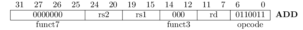
The table above shows the position and value of different fields within the instruction word. First of all, there is the opcode, located in the lower 7 bits. In case of the add instruction, its value denotes an arithmetic or logic instruction, which operates on two registers and stores the result in a register. In the RISC-V ISA, many instructions share this opcode, and the specific arithmetic or logic operation is further specified by the function fieds (funct7 and funct3). In this case, both are zero, which denotes addition. So far for the first question (what to do?). The second question (where to find the operands?) is answered by the fields rs1 and rs2, where rs means source register. The last question (where to put the result?) is finally answered by the rd (destination register) field.

As we will see in the following chapters, many of the instructions in the RISC-V base ISA share the same format as the add instruction, they are called R-type -- or register-to-register -- instructions. We will get to know a few other formats used for branches and memory instructions. But first, we will discuss the hardware components within a processor and their interconnection, which are needed to realise such instructions.